Run your impulse on a single new sample to see, window by window, what the model predicts before you deploy it.
Live classification runs your current impulse over one sample and shows you what the model predicts. The sample is usually captured from a connected device, so you can try the model on real data before you deploy it.Model testing scores your whole labeled test set and reports overall accuracy. Live classification shows the results for one sample in detail, so you can see how the model handles a specific input.
Edge Impulse moves a sliding window across the sample, using the window size and window increase configured in your impulse, runs the DSP and learning blocks on each window, and returns one result per window.Keep in mind:
Each window gets its own result. A two-second recording with a one-second window and a 100 ms increase produces around eleven results, and they can disagree with each other.
The window settings come from the impulse, so changing the window length in your impulse also changes live classification results.
Each learning block reports separately. An impulse with a classifier and an anomaly block gives you a confidence per label from the first and an anomaly score from the second, for every window.
Results are compared against the sample’s label when it has one, so you can see which windows were misclassified.
The float32 model is used by default. You can classify against the int8 model, or against several model variants at once, to see where quantization changes a prediction.
If your project has more than one experiment, live classification runs against the impulse you have selected, so switching impulses and reclassifying the same sample is a direct comparison.
Studio warns you if the sample is already in your training set. The model learned from that sample, so classify a new one to see how the model handles data it hasn’t seen.
Connect the source you want to sample from, then click Start sampling. Everything connected to your project appears under Devices.
A development board connected over the Edge Impulse CLI or WebUSB. This is the most representative option, because the data passes through the same sensor and firmware as it will in production.
Your mobile phone. Go to Devices, click Connect a new device, select Use your mobile phone, and scan the QR code. Then click Switch to classification mode and start sampling.
Your computer. Go to Devices, click Connect a new device, select Use your computer, and grant the browser access to your microphone or camera. Then click Switch to classification mode and start sampling.
Connected devices available for live classification.
Connecting a mobile phone for live classification.
You can also classify a sample that is already in your project, or upload a file, so you can rerun the same input without recapturing it.
If a model behaves differently on your device than in Studio, sample from the device itself rather than from your phone. Differences in sensor placement, sample rate, or mounting can make the device’s data look different from your training data.
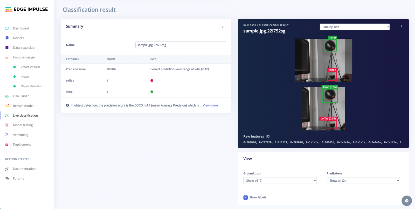
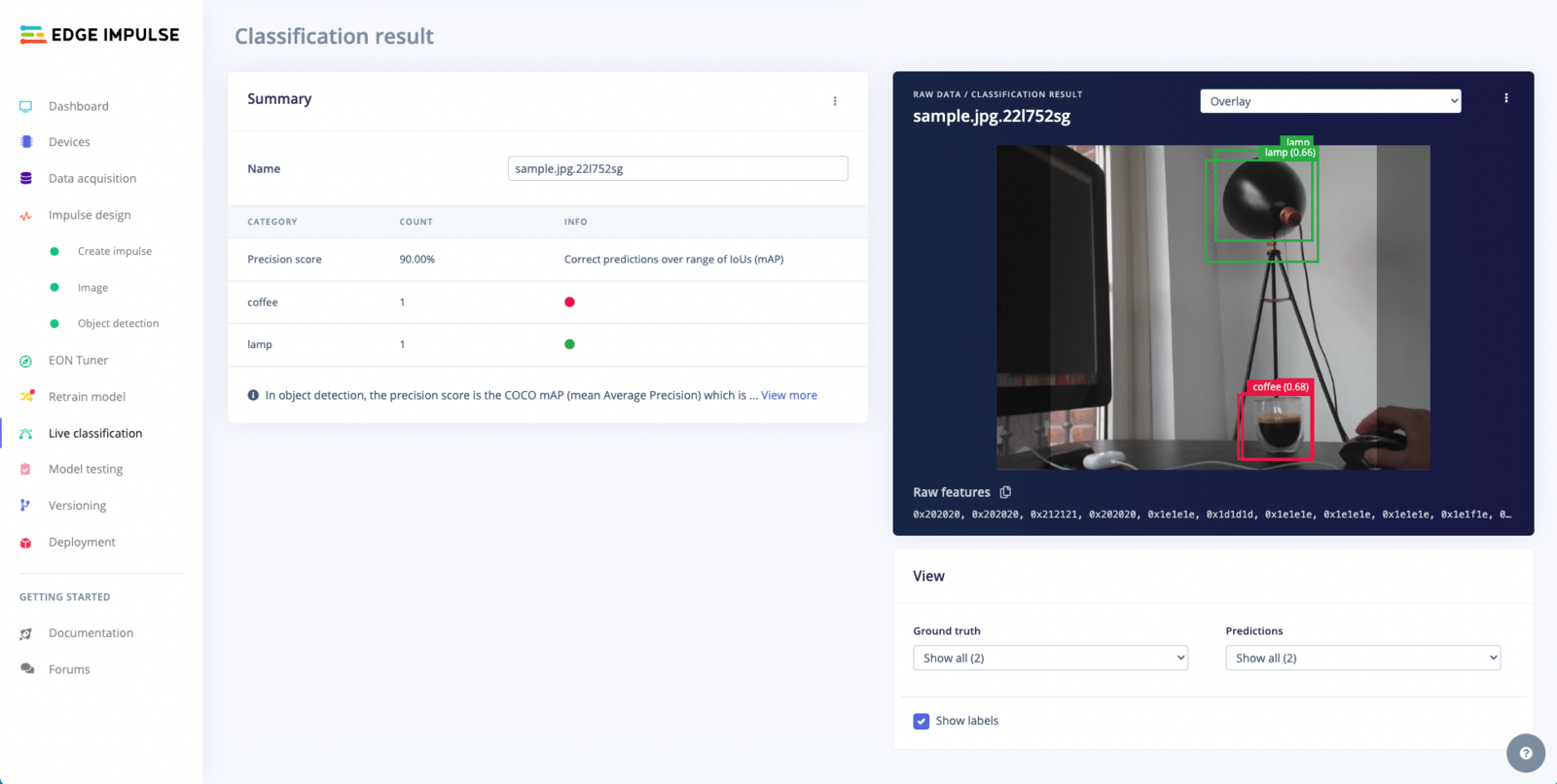
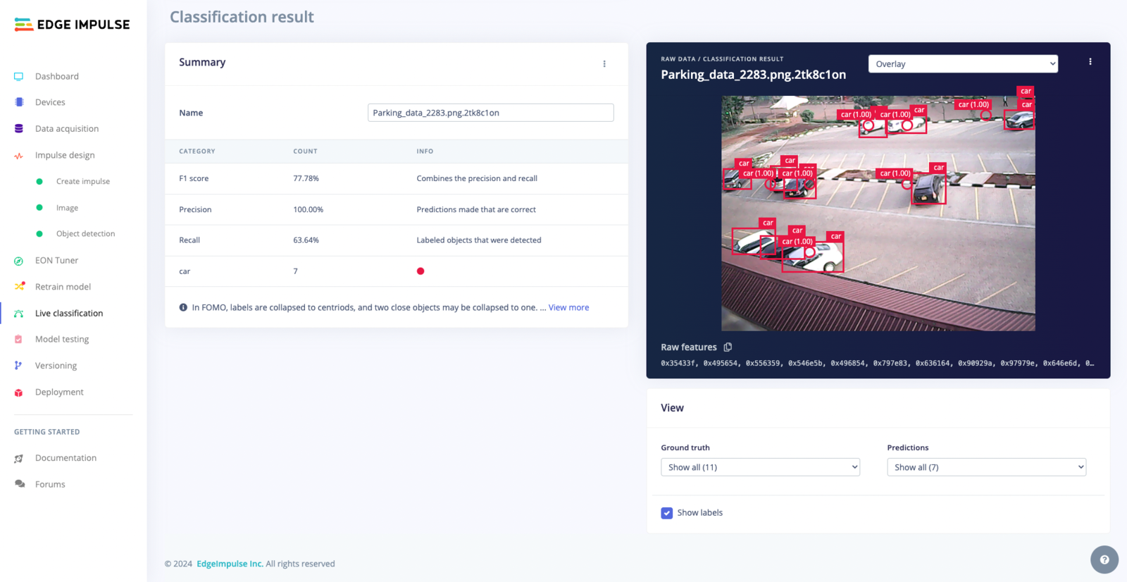
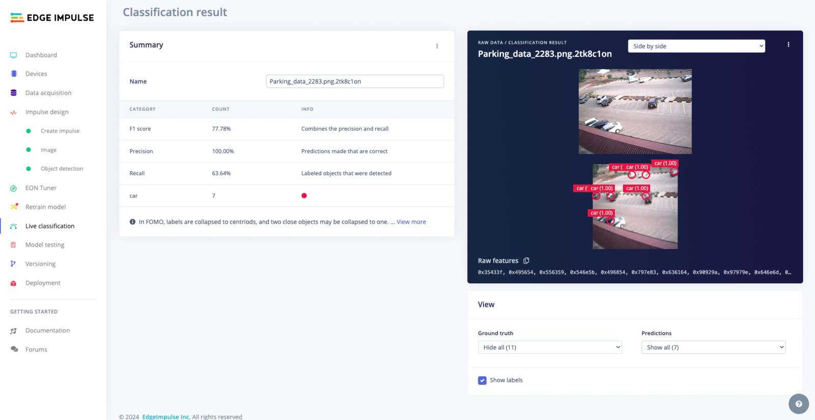
Object detection projects show detections rather than a confidence per label. Use the dropdown above the image to switch between the Side by side and Overlay views.
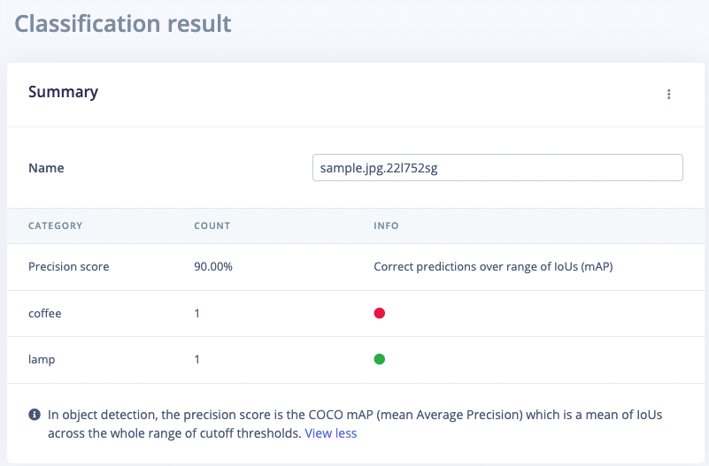
SSD MobileNet V2
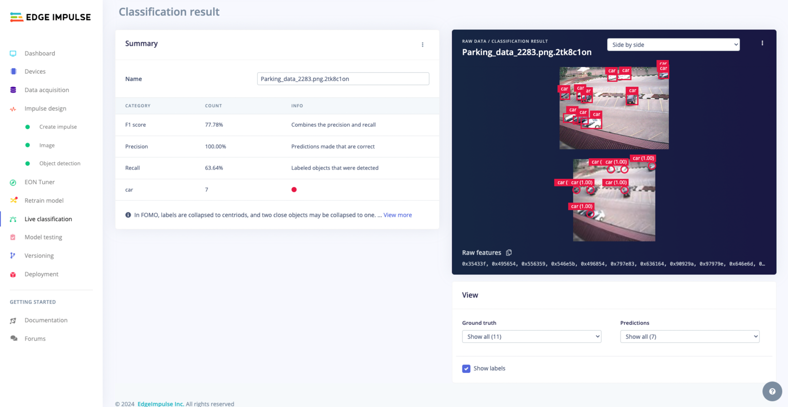
FOMO
Employs a Single Shot MultiBox Detector (SSD) with a MobileNet V2 backbone for object detection. This model is optimized for running on MCUs and CPUs.
The labeled ground truth above the model's predictions.
The top image shows the ground truth labels and the bottom image shows the predicted bounding boxes, each with a class and a confidence score. Comparing the two makes it easy to spot objects the model missed.
Bounding boxes are drawn directly on the image, with labels and confidence scores in context. Use this view to check how closely the boxes fit the objects.
The labeled ground truth above FOMO's centroid predictions.
In the image above, the model found 7 of the 11 labeled cars. FOMO predicts centroids rather than boxes, so check whether each object was found and counted.
Recall is how many of the objects actually present were found.
High precision with low recall means the model is missing objects. High recall with low precision means it is detecting objects that aren’t there. Check both numbers together.